深度学习(5)：TensorFlow

每次都从零开始全部靠自己去建立一个深层神经网络模型并不现实，借助现在众多流行的深度学习框架，能够高效地实现这些模型。TensorFlow便是其中之一。

TensorFlow

TensorFlow是Google基于DistBelief进行研发的第二代人工智能学习系统，是一个使用数据流图进行数值计算的开源软件库。其命名来源于本身的运行原理，Tensor(张量)意味着N维数组，Flow（流）意味着基于数据流图的计算，TensorFlow便意为张量从流图的一端流动到另一端计算过程。TensorFlow 中包含了一款强大的线性代数编译器XLA，这可以帮助TensorFlow代码在嵌入式处理器、CPU（Central Processing Unit）、GPU（Graphics Processing Unit）、TPU（Tensor Processing Unit）和其他硬件平台上尽可能快速地运行。

版本选择

TensorFlow分为CPU版和GPU版。GPU版需要有NVIDIA显卡的支持，TensorFlow程序通常在GPU上的运行速度明显高于CPU，查看设备是否配备了NVIDIA显卡方法另寻。

如果设备配备了NVIDIA显卡，还需根据显卡的具体型号，到NVIDIA官方文档上找到你的GPU，查看其该型号的N卡是否支持CUDA（Compute Unified Device Architecture），以及CUDA算力（Computer Capability）。TensorFlow要求GPU的CUDA计算能力值达到3.0以上，否则比直接CPU上运算的效果相差不大。一些年份较早或比较低端的显卡达不到这个要求，这种情况下即使安装了GPU版本也还是会调用CPU运算，不会调用GPU。

安装

TensorFlow的Python版本一般直接使用pip命令进行安装，CPU版本的pip安装命令为：

pip install --upgrade tensorflow

GPU版本为：

pip install --upgrade tensorflow-gpu

安装GPU版本后想要用N卡正常运行，需要先安装CUDA® Toolkit和cuDNN，根据各自的平台进行下载安装。而且需要注意，下载安装的版本务必按照安装好的TensorFlow支持的版本来。

测试

安装完成后，打开在命令行或终端中激活Python，输入以下代码：

# Python
import tensorflow as tf
hello = tf.constant('Hello, TensorFlow!')
sess = tf.Session()
print(sess.run(hello))

安装无误的话，最后将打印出熟悉的“Hello, TensorFlow!”。此外，如果安装的是GPU版，输入第三行代码后将显示你的GPU配置信息。

实现MNIST手写数字识别

MNIST数据集

MNIST（Mixed National Institute of Standards and Technology database）是一个入门级的计算机视觉数据集，其中包含各种手写数字图片：

上面的四张图的标签（labels）分别为5,0,4,1。

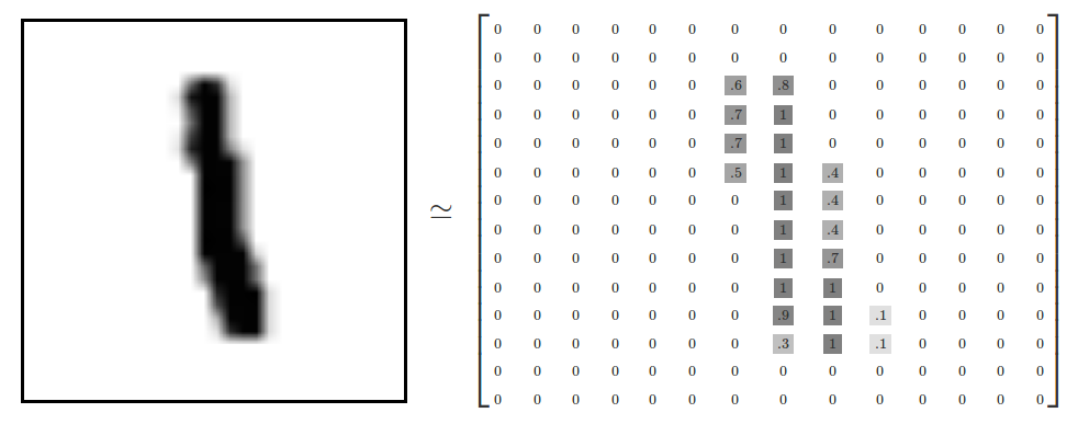
MNIST数据集被分为三部分：55000个训练样本（mnist.train),10000个测试样本（mnist.test),5000个验证集（mnist.validation)。每个样本由两部分组成，一个大小为28*28的手写数字图片像素值矩阵$x$以及它的标签$y$，标签$y$是用one-hot向量表示的，一张数字图片中的真实数字值n,将表示成一个只在第n维度的数字为1的10位维向量。例如，标签3用one—hot向量表示为$[0,0,0,1,0,0,0,0,0,0]$。one-hot编码多用在多分类问题上。

则整个训练样本中$X$（mnist.train.images）的大小为55000*784,$Y$（mnist.train.labels)的大小为55000*10。其中的数据都已经进行过标准化。

Softmax回归

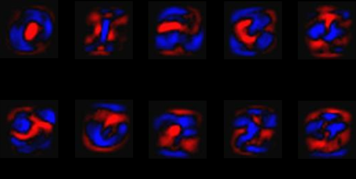
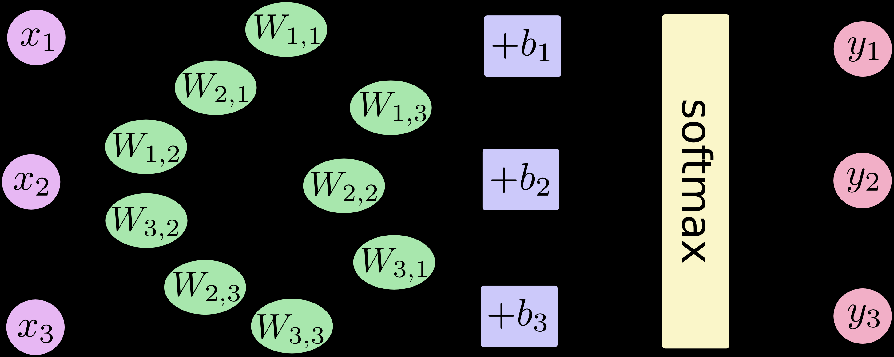
Softmax回归模型是Logistic回归模型在多分类问题上的推广。为了收集证据以便将给定的图片划定到某个固定分类，首先对图片的像素值加权值w并求和，如果有很明显的证据表明一张图片中某些像素点会导致这张图片不属于这一类，则相应的权值为负数，反之权值为正。如下图所示，其中红色部分代表负数权值，蓝色部分代表正数权值。

训练过程中，为了排除输入中引入的干扰数据，还需要设定额外的偏执量b。其实就是进行简单的线性拟合：$${ \text{evidence} = w^TX + b}$$
其中参数矩阵$w$的大小为784*10,$b$的大小为10*1。和Logistic回归一样，其中的$w$、$b$还是直接初始化为0。

Softmax回归中，激活函数使用的是softmax函数：$$\sigma(z)_{j}=\frac{e^{z_{j}}}{\sum_{i=1}^m e^{z_{i}}}$$
损失函数也变为：$$\mathcal{L}(\hat y, y) = - \sum^m_{i=1}y_i \log \hat y$$
随后使用小批量梯度下降法来求得参数的最优解。

tensorflow实现

使用tensorflow来实现这个模型：

#导入要用到的库
import tensorflow as tf
from tensorflow.examples.tutorials.mnist import input_data

mnist = input_data.read_data_sets("MNIST_data/", one_hot = True) #导入数据集

#初始化参数
W = tf.Variable(tf.zeros([mnist.train.images.shape[1],10])) #W初始化为0
b = tf.Variable(tf.zeros([10])) #b初始化为0
costs = []

#建立模型
x = tf.placeholder(tf.float32, [None, mnist.train.images.shape[1]])
y = tf.placeholder(tf.float32, [None, 10]) #建立训练集占位符

y_hat = tf.nn.softmax(tf.matmul(x,W) + b) #softmax激活
cost = tf.reduce_mean(-tf.reduce_sum(y * tf.log(y_hat), reduction_indices=[1])) #成本函数
train_step = tf.train.GradientDescentOptimizer(0.5).minimize(cost) #梯度下降，最小化成本

sess = tf.InteractiveSession() #创建session
tf.global_variables_initializer().run() #初始化变量（声明了变量，就必须初始化才能用）

#迭代运算
for epoch in range(1000):
    batch_xs, batch_ys = mnist.train.next_batch(100) #每次使用100个小批量数据
    sess.run([train_step, cost], feed_dict = {x: batch_xs, y: batch_ys}) #进行训练

#计算准确率
correct_prediction = tf.equal(tf.argmax(y_hat,1), tf.argmax(y,1))
accuracy = tf.reduce_mean(tf.cast(correct_prediction, tf.float32))
print(sess.run(accuracy, feed_dict={x: mnist.test.images, y: mnist.test.labels}))

最后用训练样本测试的准确率为92%左右。

实现手势数字识别

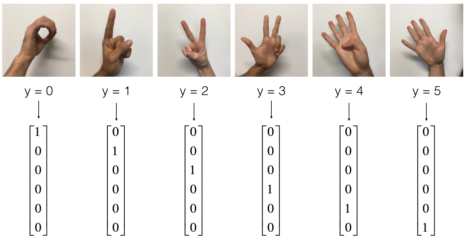
手势数字数据集中，训练样本有1080张图片，测试样本有120张图片，其中有代表着0-5的六种图片。每个原始样本由两部分组成，一个大小为64*64的手势数字图片像素值矩阵$x$以及它的标签$y$，原始样本的标签$y$是直接用手势图片表示的数字真实值表示的，还需要将它们转换为one-hot向量进行表示。

1.导入数据

#导入数据
def load_dataset():
    train_dataset = h5py.File('train_signs.h5', "r")#训练集
    train_set_x_orig = np.array(train_dataset["train_set_x"][:])
    train_set_y_orig = np.array(train_dataset["train_set_y"][:])

    test_dataset = h5py.File('test_signs.h5', "r")#测试集
    test_set_x_orig = np.array(test_dataset["test_set_x"][:])
    test_set_y_orig = np.array(test_dataset["test_set_y"][:])

    classes = np.array(test_dataset["list_classes"][:])

    train_set_y_orig = train_set_y_orig.reshape((1, train_set_y_orig.shape[0]))
    test_set_y_orig = test_set_y_orig.reshape((1, test_set_y_orig.shape[0]))

    return train_set_x_orig, train_set_y_orig, test_set_x_orig, test_set_y_orig, classes

2.one-hot编码

编码方式如图：

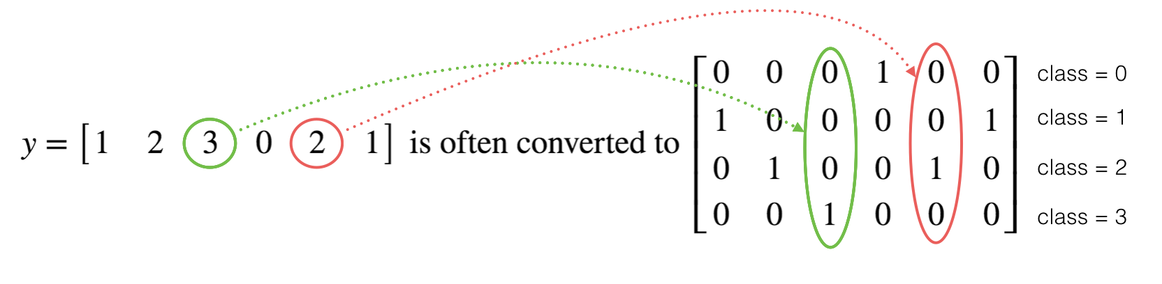
代码实现：

#ong-hot编码
def convert_to_one_hot(Y, C):
    Y = np.eye(C)[Y.reshape(-1)].T#np.eye():生成单位矩阵
    return Y

3.前向传播

#前向传播
def forward_propagation(X, parameters):

    W1 = parameters['W1']
    b1 = parameters['b1']
    W2 = parameters['W2']
    b2 = parameters['b2']
    W3 = parameters['W3']
    b3 = parameters['b3']

    Z1 = tf.add(tf.matmul(W1,X),b1)                                           
    A1 = tf.nn.relu(Z1)                                             
    Z2 = tf.add(tf.matmul(W2,A1),b2)                                             
    A2 = tf.nn.relu(Z2)                                            
    Z3 = tf.add(tf.matmul(W3,A2),b3)                                                 
    return Z3

4.成本计算

#成本计算
def compute_cost(Z3, Y):

    logits = tf.transpose(Z3)
    labels = tf.transpose(Y)

    cost = tf.reduce_mean(tf.nn.softmax_cross_entropy_with_logits(logits = logits, labels = labels))
    return cost

5.整个模型

def model(X_train, Y_train, X_test, Y_test, learning_rate = 0.0001, num_epochs = 1500, minibatch_size = 32, print_cost = True):

    ops.reset_default_graph()  #使重新运行时不覆盖tf的变量
    tf.set_random_seed(1)                             
    seed = 3                                          
    (n_x, m) = X_train.shape                          
    n_y = Y_train.shape[0]                            
    costs = []                                        

    X, Y = create_placeholders(n_x, n_y) #占位符
    parameters = initialize_parameters() #初始化参数
    Z3 = forward_propagation(X, parameters) #前向传播
    cost = compute_cost(Z3, Y) #损失计算
    optimizer = tf.train.AdamOptimizer(learning_rate = learning_rate).minimize(cost) #使用Adam梯度下降

    init = tf.global_variables_initializer() #变量初始化

    with tf.Session() as sess:

        sess.run(init) #运行变量初始化

        for epoch in range(num_epochs):

            epoch_cost = 0. #每epoch一次后的成本值
            num_minibatches = int(m / minibatch_size) #小批量数目
            seed = seed + 1
            minibatches = random_mini_batches(X_train, Y_train, minibatch_size, seed) #随机小批量

            for minibatch in minibatches:

                (minibatch_X, minibatch_Y) = minibatch
                _ , minibatch_cost = sess.run([optimizer, cost], feed_dict={X: minibatch_X, Y: minibatch_Y})
                epoch_cost += minibatch_cost / num_minibatches

            if print_cost == True and epoch % 100 == 0:
                print ("%i epoch 后的成本值 : %f" % (epoch, epoch_cost))
            if print_cost == True and epoch % 5 == 0:
                costs.append(epoch_cost)

        plt.plot(np.squeeze(costs))
        plt.ylabel('cost')
        plt.xlabel('iterations (per tens)')
        plt.title("Learning rate =" + str(learning_rate))
        plt.show()

        parameters = sess.run(parameters)
        print ("参数训练完毕")

        correct_prediction = tf.equal(tf.argmax(Z3), tf.argmax(Y))

        accuracy = tf.reduce_mean(tf.cast(correct_prediction, "float"))

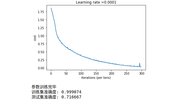
        print ("训练集准确度:", accuracy.eval({X: X_train, Y: Y_train}))
        print ("测试集准确度:", accuracy.eval({X: X_test, Y: Y_test}))

        return parameters

6.得出结果

#数据集处理
X_train_orig, Y_train_orig, X_test_orig, Y_test_orig, classes = load_dataset()
X_train_flatten = X_train_orig.reshape(X_train_orig.shape[0], -1).T #转置
X_test_flatten = X_test_orig.reshape(X_test_orig.shape[0], -1).T
X_train = X_train_flatten/255. #标准化
X_test = X_test_flatten/255.
Y_train = convert_to_one_hot(Y_train_orig, 6) #变为one-hot形式
Y_test = convert_to_one_hot(Y_test_orig, 6)

parameters = model(X_train, Y_train, X_test, Y_test)

结果为：

参考资料

1. 吴恩达-改善深层神经网络-网易云课堂
2. Andrew Ng-Improving Deep Neural Networks-Coursera
3. tensorflow官网
4. tensorflow中文社区
5. tensorflow环境搭建教程（Windows）
6. tensorflow环境搭建教程（Ubuntu）
7. 课程代码与资料-GitHub

注：本文涉及的图片及资料均整理翻译自Andrew Ng的Deep Learning系列课程，版权归其所有。翻译整理水平有限，如有不妥的地方欢迎指出。

---

更新历史：

• 2017.10.15 完成初稿
• 2018.02.13 调整部分内容